Part 3 - Introduction to neural learning and Gradient Descent
As we know the basic paradigm of DL i.e. Predict, compare, and Learn, and we already saw a few basics of prediction in part 2 so let’s get started with compare.
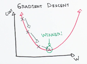
Imagine a blindfolded person who wants to climb up a mountain or go down a mountain, then he needs to tak ebig steps initally and then he need to reduce hos step size so that he don’t overshoot his final point. Some similar thing happens with Gradient. Check this blog to know more about Gradient.

So comparing gives a measurement of how much a prediction “missed” by.
Handling error is one of the crucial and tough tasks in DL because once we predicted the value it will only tell us about the amount by which it differs from the actual value i.e. - very little, a lot, perfectly predicted. And once we find out the correct error then we can move to the next step i.e. learn. In the next step, learning tells each weight that how much they can change to reduce the error. This step is all about playing a blame game, where we need to find the contribution of each weight into the error One such blame game is Gradient Descent.
Compare: Does your network make good predictions?
Let’s first understand some points -
-
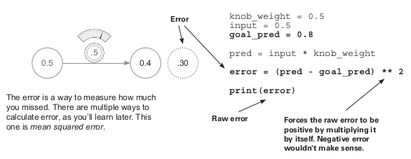
goal_pred - As we have an input that is recorded from real observation, similar to that it is the data collected from real observation for the output, for example - whether a batsman hit a century given his batting average.
-
Why is error squared - As let’s assume the archer hitting the target when the shot is 5 inches down then the error will be 5 inches. Similarly, if the sot is 5 inches up then again the error will be 5 inches. So the primary reason to square the error is because it forces the output to be positive.

Here you might think the small error(<1) will get smaller and the large error(>1) might become larger, so it happens and we pay attention to big errors and not worry much about the small ones.
Why measure error
Our main goal for measuring the error because once we have the error then we can minimize it and predict more accurately. We prioritize errors differently like we can apply MSE so that the small errors become irrelevant and only the big ones counted as a significant error.
Our main goal for accurate prediction is to make the average error close to zero. Also, we keep the error as positive because let’s assume if we have an error of +1 and then an error of -1, so the net error will be 0. So we won’t get an actual error instead wi\e’ll think we predicted perfectly.
Hot and cold Learning
Hot and cold learning means adjusting or wiggling the weights to see which direction reduces the error the most, moving the weights in that direction, and repeating until the error gets to 0.
So basically we first make the weight down and then up and finally we can decide whether to increase the weight or decrease the weight to make the prediction more accurate. In actual NN we need to perform this step many times to find the correct weights.

Characteristics of Hot and Cold learning -
- Simple - It’s simple like you just need to make your weight slightly high or less than compare the error of each case with the current error, based on that take the decision to increase or decrease the error.
- Problem 1: Inefficient - We need to predict multiple times to update the knobs.
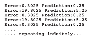
- Problem 2: Hard to predict exact goal prediction - We need to set the step_amount carefully otherwise it will overshoot the output or maybe just oscillate between some values. For example, in the previous case if the step_amount is 10 then the image would be something like this -

Not only the amount we also need to decide the direction where we want to go. It’s also inefficient because it calculates the prediction thrice for each weight update and arbitrary step_amount (down_weight, same weight, up_weight)
Calculating both direction and amount from error
Let’s get first discuss this -
- direction_and_amount - It represents how you want to change weitght, the first part is pure error and the scond part is scaling, negative reversal, and stopping.
- Pure error - The pure error is ( pred - goal_pred ), which indicates the raw direction and amount you missed. If this is a positive number, you predicted too high, and vice versa. If this is a big number, you missed by a big amount, and so on.
- Scaling, negative reversal, and stopping - These three attributes have the combined effect of translating the pure error into the absolute amount you want to change weight . They do so by addressing three major edge cases where the pure error isn’t sufficient to make a good modification to weight .
- Stopping - Stopping is the simplest effect on the pure error cuase by mltiplying it by input. If input is zero then the direction_and_amount will become 0, because there’s nothing to learn. For example - imagine plugging a CD player into your stereo. If you turned the volume all the way up but the CD player was off, the volume change wouldn’t matter.
- Negative reversal - This is probably the most difficult and important effect. Normally (when input is positive), moving weight upward makes the prediction move upward. But if input is negative, then all of a sudden weight changes directions! When input is negative, moving weight up makes the prediction go down. It’s reversed! How do you address this? Well, multiplying the pure error by input will reverse the sign of direction_and_amount in the event that input is negative. This is negative reversal, ensuring that weight moves in the correct direction even if input is negative.
- Scaling - Logically if input is big then the update in weight will be big, sometimes it has cons also like it goes out of control, for that we’ll discuss alpha.
Gradient Descent
As I told in the beginning about a blindfolded person. There is some similarity in Gradient Descent also, here as we need to minimize the error so we plot a graph between error and weight (reference - check part 2), here our aim is to minimize the error i.e. to reach to minimum point, also we need to take care that the NN should not overshoot that point.

Here we update our parameters like weight. So first we predict the value then we calculate the loss/error, and then we calculate the delta factor and apply the previous scaling, reversal, and stopping technique to calculate the weight_delta and finally we multiply it by alpha and update our parameters.
Steps -
- Predict
- Calculate error/loss (predict-actual)
- Calculate weighted delta -
- Pure error
- Scaling, stopping, and reversal
- Multiply it with alpha and update the weight (parameters)
i.e.
for iteration in range(4):
		#Next two lines have the secret.
		pred = input * weight
		error = (pred - goal_pred) ** 2
		delta = pred - goal_pred
		weight_delta = delta * input
		weight = weight - weight_delta
		print("Error:" + str(error) + " Prediction:" +
				str(pred))
Learning is just reducing errors
All you’re trying to do is figure out the right direction and amount to modify weight so that error goes down. We can replace the actual pred formula and value of goal_pred in the error formula which will make the equation something like this (assume input = 0.5 and goal _pred = 0.8)-
$error = ((0.5*weight) - 0.8)**2$
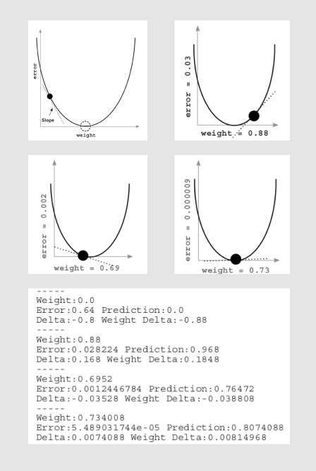
Here we can see this is a quadratic equation between error and weight, So we can use the slope to reduce the error and jump to the minimum point i.e. The slope points to the bottom of the bowl (lowest error ) no matter where you are in the bowl. You can use this slope to help the neural network reduce the error.
Here you may think, we can change weight, input, goal_pred, **2, or other arithmetic calculations, but this is not true if we change input or goal_pred then we are seeing the world as we want to see not as it is. Similarly changing the arithmetic will just change how we calculate the error, so we need to make sure that it should give good measure. So the only possible way to tweak the prediction is to adjust the weight or the knobs to reduce the error to 0.

So now we know learning is just adjusting the weight so that the error is reduced to 0. So for this, we need to understand the relationship between error and weight. We saw the equation i.e.
$error = ((input * weight) - goal_pred) ** 2$
so by the help of this equation, we can define the relation between weight and error(other parameters not changing).
With the help of this equation, we can find that the derivative will be of linear order and if we plot the graph for error vs weight then we’ll get the parabola in which the lowest point will show the minimum error for a particular weight. If we check the rate of change of error w.r.t. weight then we’ll find that on the left side the derivative of the slope is always negative and right side the derivative of the slope is always positive. So we can use this idea to go down to the minimum point where the error is zero.
A derivative gives you the relationship between any two variables in a function. You use the derivative to determine the relationship between any weight and error. You then move the weight in the opposite direction of the derivative to find the lowest weight. This method is called gradient descent, here you move the weight value opposite the gradient value, which reduces the error to 0 i.e. if we increase the weight when you have a negative gradient and vice versa.
If the input is sufficiently large then the update in the weight would be larger even if the error is small. The network overshoots i.e. divergence. If we have a big input then the prediction would be more sensitive to the changes in the weight. So for this, we can use alpha.
Intro to alpha
As in the last problem when the input is large then the weight update can overcorrect. This happens because every time the change or derivative magnitude is larger than the previous one. The general problem we can see is every time this big change it overshoots the minimum point. So we can take a fraction of this derivate by multiplying it with alpha (value between 0 or 1). Not only for big input we can still use it for small inputs to reduce the weight updates.
Finding the appropriate alpha is the state of art in neural networks, it’s often done by guessing. We watch the error and based on that we define whether to increase or decrease alpha. If the learning is very slow then we need to increase the alpha and if there is some overshoot issue then we can decrease the alpha.
So in next blog we’ll see more about Gradient Descent and backward propagation….
Enjoy Reading This Article?
Here are some more articles you might like to read next: