Introduction to Adversarial ML

Hi all, let’s see an interesting case, picture this: you’ve trained a machine learning model to identify images of dogs and cats accurately. It’s performing great during testing and you’re excited to deploy it in the real world. But what happens when someone tries to trick the model by feeding it with images that are slightly altered, making it misclassify them?

With the increasing prevalence of AI-assisted tools and the upcoming deployment of AI in real-world use cases, it’s crucial that we shift our focus beyond performance metrics and prioritize the robustness of these models. One observation I’ve made is that we tend to emphasize improving accuracy or other metrics when developing ML models. For example, if you’re an ML enthusiast who has created models for classification or segmentation tasks, you’re probably measuring the model’s performance based on its accuracy or F1 score. However, we need to take into account additional factors to ensure the model doesn’t fail in real-world scenarios.

Think about it - what if a camera installed at a busy intersection failed to count the number of cars crossing the road due to external disturbances like weather or background noise? Or worse, what if someone could easily trick a face recognition system with a patch that looks similar to your face? These scenarios highlight the pressing need to make AI systems more secure and resilient to such corruption. These corruptions could be Adversarial attacks, in which an attacker intentionally manipulates data to mislead or evade AI systems, which are one example of the potential risks associated with AI. Additionally, AI systems can potentially reveal sensitive personal information if they are not properly secured.

As I delved deeper into the realm of AI security and privacy, I was surprised to find very less resources to read more on this topic. That’s why I’ve decided to start a conversation on Adversarial ML - a specific area of privacy and security that deals with protecting AI systems from adversarial attacks. Let’s dive in!

I would suggest before diving deeper into Adversarial ML, you should have a certain level of familiarity with fundamental deep learning concepts such as optimization, gradient descent, deep networks, and so on. In case you want some good resources you can check out Deep Learning Book, PyTorch Tutorials, or any resources that might be helpful to understand the underlying concepts.

So let’s start but before that why not talk about a few terminologies that we are going to use throughout the series?

What are adversarial attacks -

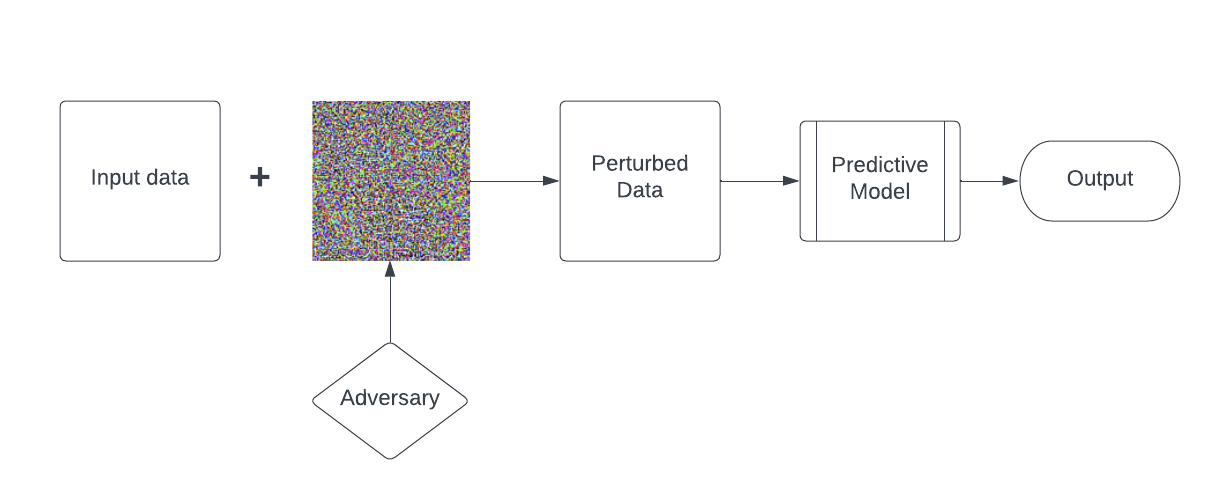
An adversarial attack is a technique used to intentionally manipulate or trick a machine learning model by introducing carefully crafted input called perturbations that are designed to cause the model to produce incorrect output or in general misclassify the labels. Adversarial attacks can take many forms, but some common examples include adding imperceptible noise to an image or text input, modifying a small subset of the input data, or changing the distribution of the input data. Adversarial attacks are a concern in many machine learning applications, such as computer vision, natural language processing, or speech models.

Difference between Targeted and Untargeted attack: In the case of a non-targeted attack, the generated adversarial images can be assigned to any class but on the other hand, targeted adversarial images are specific to particular classes.

Difference between White box and Black Box attack: A white box attack is an attack scenario where the attacker has access to the target model such as its model’s architecture and its parameters. On the other hand, a black box attack is an attack scenario where the user has no access to the model but can only access inputs and observe the outputs.

There are two other important methods of attack such as backdoor attack (poisoning) and Gradient-based attack. In the first case, the attacker has access to the network learning process and the training data, and in the latter one, the attacker tries tricking an already trained model by generating adversarial examples from the inputs.

So in this blog let’s first discuss the gradient-based attack.

Let’s begin by exploring some practical applications while simultaneously learning the relevant theory. I will be incorporating some mathematical concepts along the way, which may significantly enhance the complexity of the topic. However, I will try to provide relevant links and explanations to ensure that it remains clear and understandable.

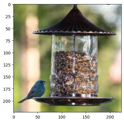
To start, I will use a pre-trained ResNet18 model by PyTorch to classify the image of a Indigo

from PIL import Image
from torchvision import transforms

indigo_img = Image.open("indigo.jpg")
preprocess = transforms.Compose([
   transforms.Resize(224),
   transforms.ToTensor(),
])
indigo_tensor = preprocess(indigo_img)[None,:,:,:]
plt.imshow(indigo_tensor[0].numpy().transpose(1,2,0))

Now we have the image next we need a model, so let’s load the model, in my case I am using a pre-trained ResNet18 model by PyTorch. You can also train your own model based on your use case.

import torchvision.models as models
model = models.resnet18(pretrained = True)
model.eval()

And for prediction -

#Applying normaliztion
trans = transforms.Compose([
   transforms.Normalize((0.485, 0.456, 0.406), (0.229, 0.224, 0.225)),  
])
output = model(trans(indigo_tensor))
pred = output.argmax(dim = 1, keepdim = True)

To be sure let’s confrim the predicted label first -

import json
    with open("/content/imagenet-simple-labels.json") as f:
        imagenet_classes = json.load(f)
    print(imagenet_classes[pred.item()])

Ok everything is working fine our model predicted correctly that it is a Indigo. Now next we need to generate the perturb data. So before that let’s come to some general concepts of model. So we have input space X (say), and the output space will be a k dimensional vector space (k being the number of classes), here the output space vector could be the logit space. So we can define the function for the model something like -

Here 𝜃 represents parameters that we typically optimize when we train a neural network. So finally we can say h𝜃 corresponds to the model.

Now the other important thing that we optimize is the loss during the training. Now as we all know to calculate loss we need the predicitons and true labels or the ground truth. So we can define our loss as -

here x ∈ X and y ∈ Z, where Z is nothing but the true class. In short we can also say \(l: \mathbb{R}^k \times \mathbb{Z}_+ \rightarrow \mathbb{R}_+\)

it means, loss it nothing but a mapping from the model predictions and the ground truth to a non-negative number (loss value). There are several loss funciton we can use such as log loss, hinge loss, MSE, etc. Let’s understand in terms of cross entropy loss. Thw whole idea of training a network is to maximize the probability od the actual class out of all the other classes. We all know as we apply a softmax activation to get the probability distribution which is defined as -

Also the probabilities are too small so we focus more on log of the probability of the true class which is -

And then rather than maximizing the probability distribution we can minimize the loss which is nothing but the negation of the above equation which is -

too much maths but for our use case we can simple use this function by PyTorch to use the cross entropy loss -

import math
# [14] is the class of Indigo
loss = nn.CrossEntropyLoss()(output,torch.LongTensor([14])).item()
probability = math.exp(-loss)
print (f"Loss: {loss}, probability of class Indigo: {probability}")

Output: 
Loss: 0.05189608410000801, probability of class Indigo: 0.9494275223323242

So if apply exp of this we an approximately as probability which is a good accuracy.

Now let’s learn how to create the adversarial example

Generating an adversarial example

Our main aim is to manipulate the input image which will make the model to misclassify the image or believe it is something else. So let’s understand why we want to craft perturbation in the input data. As we know for good training we need to minimize the loss such that the model performs well on inputs which we achieve by gradient descent for some minibatch $\beta$ where we compute the gradient of our loss w.r.t. parameters 𝜃 i.e.

Here the interesting part is the gradient ($\Delta_\theta l(h_\theta(x_i),y_i)$), it compuates how the small change in $\theta$ will affect the loss and overall probability. This parameter update is done using the efficient backpropagation algorithm. Here in this we can also compute the effect on loss due to input change i.e. change in loss w.r.t. input $x_i$. So we can make small changes in the input which will overall affect the loss and hence the prediction. So in case of training we update the parameters in such a way so that we minimize the loss but in our case to generate the adversarial example we’ll maximize that loss which makes our optimization problem as -

here $\hat{x}$ denotes the adversarial example which is trying to maximize the loss. Now comes the important point, what if we replace this image with some other image let say tigershark (in our case). The model will then misclassify the label. In this case we didn’t fool the classifier. So we need to make sure that $\hat{x}$ is close to our original inout $x$. So by convention we can say we can add a specific amount of perturbation in the sample let say $x + \delta$ and this $\delta$ can vary through $\Delta$. So now our optimisation equation is going to be -

Now comes the other important topic of discussion i.e. how to decide for this $\Delta$ i.e. allowed set of perturbation. In simple langauge this value can be anything which when added to the actual image, human visually feel no difference with the original input image. So we can apply several types of transformations in the image keeping in mind that it should not affect the semantic content of the image under the added perturbation. Mathematically we define a perturbation set which can be L norms such that we need to bound the added perturbation inside the L norms ($ L_0, L_1, L_2, or L_\infty s$). The most common is $L_\infty$ ball. $L_\infty$ norm for vector a is defined as -

which means it refers to the maximum absolute value of the elements in a vector $a$. So while adding the perturbation in the image we need to take care that the magnitude lie between $[-\epsilon, \epsilon]$. Also we need to make sure that if the iamge is normalised i.e. if all pixel lie between $[0, 1]$ then we need to make sure that $x + \delta $ lie between the same range too. But first let’s see a basic example of attacking a model.

import torch.optim as optim
epsilon = 2./255
#adversarial perturbation
adv_per = torch.zeros_like(indigo_tensor, requires_grad=True)
opt = optim.SGD([delta], lr=1e-1)

for ite in range(50):
    pred = model(trans(indigo_tensor + adv_per))
    loss = -nn.CrossEntropyLoss()(pred, torch.LongTensor([14]))
    if ite % 10 == 0:
        print(f'{ite}: {loss.item()}')
    
    opt.zero_grad()
    loss.backward()
    opt.step()
    adv_per.data.clamp_(-epsilon, epsilon)
    
print("True class probability:", nn.Softmax(dim=1)(pred)[0,14].item())

Output:
0: -0.05189608410000801
10: -21.462343215942383
20: -26.89446258544922
30: -28.595821380615234
40: -27.62549591064453
Indigo class probability: 1.5631285328610023e-12

Let’s understand the code, here we are using the SGD optimiser for gradient optimiszation using backpropagation. Further we mentioned the value of $\epsilon$ for the making it inside the $L_{inf}$ ball. Next we are initalizing the adversarial perturbation(adv_perturbation) which is a zero tensor similar to the input image and the requires_grad=True argument specifies that the tensor will be used in a computation graph and that gradients will be computed with respect to it. Next we iterate the 50 gradient step (similar to PGD type attack). So now we’re following the same step of first finsing the prediction for image + adv_per and then calculated the loss and used the negative sign to maximize the loss by making model more confident in such predictions. Next we clear (opt.zero_grad()) previously stored gradient of the optimizer and compute the gradients of the loss w.r.t. adv_per using autograd engine. Next opt.step() will update the adv_per tensor using the gradients computed in the previous step. Over the iteration we also need to keep track that our updated adv_per lies between [$-\epsilon, \epsilon$], so for this we use data.clamp_ to achieve this.

So what did the model actually classified after adding perturbation -

max_class = pred.max(dim=1)[1].item()
print("False predicted class name: ", imagenet_classes[max_class])
print("False rredicted class probability:", nn.Softmax(dim=1)(pred)[0,max_class].item())

Output:
False predicted class name:  chickadee
False predicted class probability: 0.9999942779541016

But actually this is how chickadee looks like -

And this how our image looks like after adding perturbation to normal eyes

plt.imshow((indigo_tensor + delta)[0].detach().numpy().transpose(1,2,0))

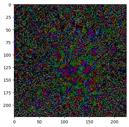
Let’s see how the adversarial perturbation looks -

This is the very fundamental implementation of adversarial attack, there are several attacked that we’ll learn in the upcoming blogs such as FGSM, PGD, BIM, Carlini Wagner, etc. You might say that the Chickadee looks similar to an Indigo, what if we want to make the image more different or say targeted towards a particular class. So we’ll see that in next blog on how to make the targeted perturbation towards a particular class.