Part 5 - Gradient Descent and Backpropagation
In the past few blogs, we saw how to deal with neural networks for example how to train, predict, and adjust the knob to decrease the error. All those neural networks had only one Layer with single or multiple inputs and output nodes. Even if you remember the last blog, we discussed one real-world dataset (MNIST), we again saw one Layer NN.
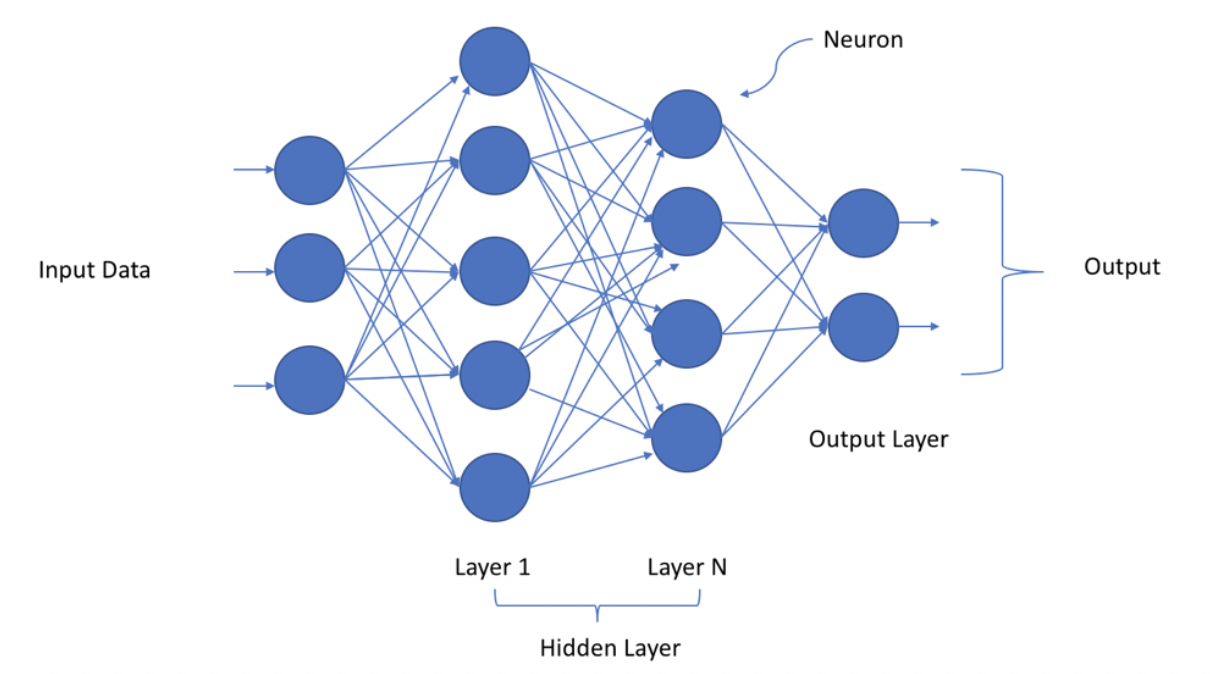
Now it’s time to dive deeper and see how deep NN works.
Let’s see a streetlight problem
Let’s assume you are some other country and you don’t know about the street signals in that country, so you planned to learn it through the actions of other people crossing the roads. So you might sit in a corner and observe the relation between the light combination and the people around you who are either walking or stopping based on the street lights.
Let’s say there are three light combinations so you need to decode the pattern and then it would be easy for you to cross the roads. Let’s discuss some of your observations (Assume if RED means OFF and BLUE means ON)
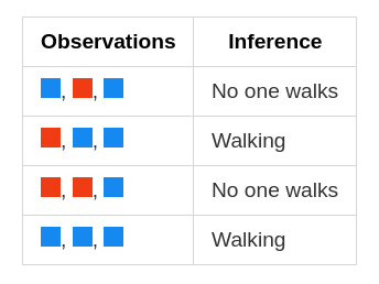
With the help of these observations, we can say that middle lights perfectly correlate with whether a person should walk or stop. This is what we generally do in a Neural Network i.e. we have some data and then we train based on that data.
Let’s prepare the data for the same example, so as we are going to make it a supervised learning problem so we need two datasets i.e. the dataset we know and the dataset we want to know. In our example as we know the street light pattern at a given time and whether the person walks or stops i.e. -
Observation = What we know & Inference = What we want to know
This is the common representation our brain understands but how do computers will understand, the answer is MATRIX. Let’s convert this to a matrix form.
Matrix - [What we know]
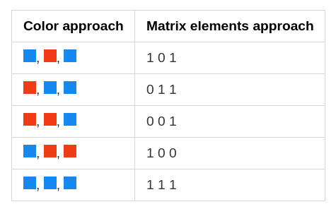
The convention is we generally represent each recorded example in a single row and each thing recorded in a single row. Not only this here we saw the data is perfectly aligned based on 1s and 0s. But it can also be managed in the data form based on the light intensities i.e. Matrix - [What we know]
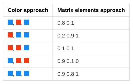
This would be more realistic recorded data. Also, we can multiply this by any constant but it will remain the same i.e. the underlying pattern would be the same. Similar to this we can also transform the matrix which we want to know into matrix form i.e. -
Matrix - [Which we want to know]
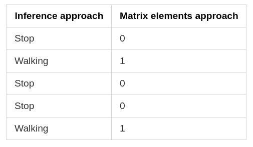
The resulting matrix in both cases is called a lossless representation as we can move back and forth based on our needs. Also, we can create these matrices with the help of NumPy as we saw in one of the last blogs. Now let’s develop a simple Neural Network (training based on each example in a neural network) based on that -
import numpy as mp
weights = np.array([0.5, 0.48, -0.7])

alpha = 0.1
streetlights = np.array( [ [ 1, 0, 1],
                           [ 0, 1, 1],
                           [ 0, 0, 1],
                           [ 1, 1, 1],
                           [ 0, 1, 1],
                           [ 1, 0, 1] ] )
walk_vs_stop = np.array( [ 0, 1, 0, 1, 1, 0 ] )
input = streetlights[0]
goal_prediction = walk_vs_stop[0]

for iteration in range(40):
    error_for_all_lights = 0
    for row_index in range(len(walk_vs_stop)):
        input = streetlights[row_index]
        goal_prediction = walk_vs_stop[row_index]
        prediction = input.dot(weights)
        error = (goal_prediction - prediction) ** 2
        error_for_all_lights += error
        delta = prediction - goal_prediction
        weights = weights - (alpha * (input * delta))
        print("Prediction:" + str(prediction))
    print("Error:" + str(error_for_all_lights) + "\n")
Types of GD
- Stochastic Gradient Descent - It updates the weight one example at a time i.e. it will take the first example and then it will try to predict and calculate the weight_delta and updates the weights and then it will move to the second example and so on. It iterates through the entire dataset many times until it finds the best weight configuration.
- Full Gradient Descent - Instead of updating the weight once for each training example, the network calculates the avg weight_delta over the entire dataset, changing the weights only each time it computes a full average.
- Batch Gradient Descent - Instead of updating the weights after just one example or after the entire dataset we select a batch size (typically between 9 and 256) of example, after which the weight got updated.
Neural Networks and Correlation
As in the last example, we knew what we are doing i..e relation between street lights and whether the person walks or stops. But what actually Neural Network understood? Did it understand the same thing we understood? For the NN it is just a pattern which it is learning i.e. how the input is correlated with the output. Or we can say it identified the correlation between middle input and the output.
So correlation works here? The basic answer is the up pressure works for middle weight and down pressure works for other weights.
What is up and Down pressure
As we know the common or shred error can be only reduced to 0 which means the network needs to figure out which weight is contributing and which is not. Let’s take the street light example again -
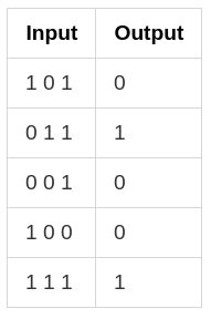
If we consider the first training example, the middle input is 0 and others are 1, but the output is 0 which means we don’t need to care for middle input now as it is 0 and any error will be only related to the left and right weight. So both the left and right input is 1 and the output is 0 which means we need to down the input so here we’ll apply down pressure. So it means in the first example there is a decorrelation between the left and right weights w.r.t. the output. The weight table would be something like this -
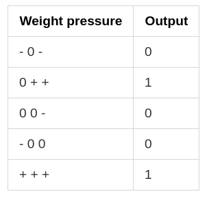
Here - indicates that there is a downward pressure, + indicated that there is an up pressure, and 0 indicates that there is no pressure. So if we see on average, the left weight has 2 negative and one positive so it will move the weight towards 0. Similarly, the middle weight has 2 positives which will move the middle weight towards 1. Each individual weight here is trying to compensate for the error. The whole process of training is that the learning algorithms reward the input which is correlating the output and penalize the input which is decorrelated with the downward pressure. The weighted sum of the inputs perfectly correlates between the input and output by weighting decorrelated inputs to 0. Let’s see some of the edge cases -
- Overfitting - Let’s again take the first example of streetlight [ 1 0 1 ] here what if the weight were 0.5 and -0.5 for far-right and far-left weights. Then the overall prediction is going to be 0 (-0.51 + 0.51 ) in this case. Here the weight is giving the prediction as 0 i.e the output we want. But is it a correct weight configuration? No right because it will fail for other real-world examples i.e. it just learned how to predict safely not how to predict originally. This is known as overfitting. The correct way is to giving the heaviest weight to the best input where it will predict the correct output not the safe one. So we need to make our neural network generalize instead of memorizing.
- Conflicting pressure - If we consider the far right column in our example then we could say that it contains equal no. of positive as well as negative i.e. equal no. of upward and downward pressure. But on the other hand, we know the weight pushes it to 0 which means downward pressure is greater than upward pressure. So here for predicting 1, we have a 1:1 relation of middle weight with the output but for predicting 0 we may get some issue. Further, we’ll also learn about regularization, as if a weight has equal down and up pressure, then it is of no use, i.e. it’s not helping in either direction. So regularization says that weight with really string correlation is going to contribute or stay, and everything else would be considered as noise.
So in these two points, we saw how correlation can be made but still, it won’t be of any use.
Also, lemme talk some more about point no. 2. So in that we took an example of the right weight, it has equal no. of up and down pressure but the other weights were contributing so we managed to reduce the error. What if we have all the weights have the same equal up and down pressure for example let say the recorded examples are something like -
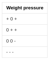
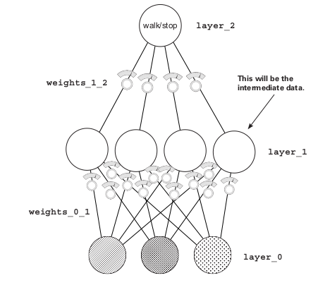
Here the problem is all three weights have an equal number of up and down pressure. So if the data doesn’t have any direct correlation then we can have intermediate data which has the connection. Till now we are using the input and output only to design a correlation so we can use some intermediate layer to fix this. For example, we can have two layers, the first one will create an intermediate dataset that has a limited correlation with the output, and the second will use that limited correlation to correctly predict the output. So it’s basically like two layers i.e. layers stacked over each other i.e. the output of the Layer_0 to Layer_1 will act as an input to the Layer_1 to Layer_2. So the whole thing is done already we know how to deal with the single-layered Neural Network and that would be similar in the stacked neural network.
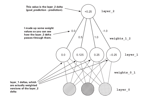
##Backpropagation The main thing why we want a two-layered network is because there is no direct correlation between the input and output so we are creating an intermediate layer to solve this issue. So if we again jump to our main aim of the neural network is that we need to reduce the error to 0, we need delta, weight delta and then update the weights to do so. Now we have the delta of Layer_2 so we can get the delta of Layer_1 by multiplying the delta of Layer_2 with the weights of Layer_1 i.e.
delta of Layer_1 = d_1
delta of Layer_2 = d_2
then d_1 = d_2*weight_1
It’s like we are applying the prediction login in reverse. This way of moving the delta signal around is called backpropagation. It basically tells us that how much nodes of Layer_1 contribute to nodes of Layer_2 or basically Layer_2 error. So you can get some idea that over the layer we are making the nodes to have some correlation with the output. And by the help of the delta of each layer, we can easily find the weight_delta and then so on.
One more common problem is we can get the same result in 2 Layer NN with whatever we are getting in 3 Layered NN because the simple logic would be 2*100*5 = 1000 and 10*100 = 1000, so we can see both have same results. Then the question is why we should use one more Layer if we are getting the same thing as it will be more expensive to calculate one more weighted sum. The answer is again related to correlation i.e. we turn off the node that has a value below 0 as we know they are not going to contribute. So if we turn it off then simply it is not going to affect the weighted sum and hence we’ll find the result based on the node which will selectively pick whether to get correlated or not. Earlier they are always correlated so sometimes they affect the results also. We use Relu to achieve it that is it will make the passed input 0 if it is less than 0. So by the help of adding one more layer, we are providing this choice that whether to subscribe for a node or not.
##First Deep Neural Network So as we discussed most of the stuff like over the layer we move in the same way as we did earlier i.e. we use the normal dot function to solve all this problem. We doing all this because we need to find which input is contributing to the final error and how to reduce it with the help of the weights. Here we also one new thing which is relu2deriv that’s only there to make the node delta 0 if the node is 0. Adjusting the weights to reduce the error over a series of training examples ultimately searches for correlation between the input and the output layers. If no correlation exists, then the error will never reach 0.
import numpy as np
np.random.seed(1)
Returns x if x > 0;
returns 0 otherwise
def relu(x):
    return (x > 0) * x
def relu2deriv(output):
    return output>0
streetlights = np.array( [[ 1, 0, 1 ],
                          [ 0, 1, 1 ],
                          [ 0, 0, 1 ],
                          [ 1, 1, 1 ] ] )
walk_vs_stop = np.array([[ 1, 1, 0, 0]]).T
alpha = 0.2
hidden_size = 4
weights_0_1 = 2*np.random.random((3,hidden_size)) - 1
weights_1_2 = 2*np.random.random((hidden_size,1)) - 1
for iteration in range(60):
    layer_2_error = 0
    for i in range(len(streetlights)):
        layer_0 = streetlights[i:i+1]
        layer_1 = relu(np.dot(layer_0,weights_0_1))
        layer_2 = np.dot(layer_1,weights_1_2)
        layer_2_error += np.sum((layer_2 - walk_vs_stop[i:i+1]) ** 2)
        layer_2_delta = (layer_2 - walk_vs_stop[i:i+1])
        layer_1_delta=layer_2_delta.dot(weights_1_2.T)*relu2deriv(layer_1)
        weights_1_2 -= alpha * layer_1.T.dot(layer_2_delta)
        weights_0_1 -= alpha * layer_0.T.dot(layer_1_delta)
    if(iteration % 10 == 9):
        print("Error:" + str(layer_2_error))
So in the next blog, we’ll learn more about correlation and Relu…
Enjoy Reading This Article?
Here are some more articles you might like to read next: