Part 4 - Gradient Descent in multiple weights
As in part 3, we saw how to update weights using Gradient descent, in this part, we’ll start and reveal how to use the same technique to update a network that contains multiple weights. Let’s see how to learn multiple weights at a time.

Mupltiple Input nodes
In the case of multiple inputs, we can use the delta i.e. (pred-true) for calculating the delta which is going to be the same for all the inputs as we only have one output which means only one pred and one true. So how we’ll get individual updates? i.e. we need to find the individual weight deltas. As we know that the weight delta = delta*input, and in our case delta is the same but as we have multiple inputs so with the help of we can easily calculate individual updates for each weight. Let’s see the example -
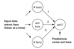
Here in this case we have 3 inputs 8.5, 0.65, and 1.2 having weights as -1.2, -0.9, and -1.7 respectively. Then further we found the delta as -0.14 which will help us to find the individual weight deltas and further it will help to find the change in weight parameters. And once we got the updated weights then we are all set to move it to around zero error in some more iterations (probably).
If you forget what is a delta and weight delta so you can check the last blog once, but as your friend, I will tell you once again in short -
- Delta (pred - true) - It is a measure that tells how much higher or lower you want a node’s value to be to predict perfectly based on the current training example. Basically, it tells us how far we are from our true output.
- Weight_delta (delta*input) - It is a derivative or basically tells us the amount and the direction you should move your weight to reduce to node_delta, accounting for scaling, negative reversal, and stopping.
So as we saw in multiple inputs, the reason for different weight updates is because of the multiple inputs.
def neural_network(input, weights):
	out = 0
	for i in range(len(input)):
	out += (input[i] * weights[i])
	return out

def ele_mul(scalar, vector):
	out = [0,0,0]
	for i in range(len(out)):
	out[i] = vector[i] * scalar
	return out

toes = [8.5, 9.5, 9.9, 9.0]
wlrec = [0.65, 0.8, 0.8, 0.9]
nfans = [1.2, 1.3, 0.5, 1.0]
win_or_lose_binary = [1, 1, 0, 1]
true = win_or_lose_binary[0]

alpha = 0.01
weights = [0.1, 0.2, -.1]

input = [toes[0],wlrec[0],nfans[0]]

for iter in range(3):
	pred = neural_network(input,weights)
	error = (pred - true) ** 2
	delta = pred - true
	weight_deltas=ele_mul(delta,input)
	print("Iteration:" + str(iter+1))
	print("Pred:" + str(pred))
	print("Error:" + str(error))
	print("Delta:" + str(delta))
	print("Weights:" + str(weights))
	print("Weight_Deltas:")
	print(str(weight_deltas))
	print(
	)
for i in range(len(weights)):
	weights[i]-=alpha*weight_deltas[i]
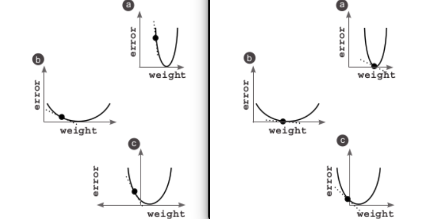
If we plot the graph of error vs weight then we can see the most of the learning or change in weight happens in the weight which has the largest input, because as we know weight delta is nothing but input*delta.
Let’s see one interesting point - what if we freeze one weight and update others
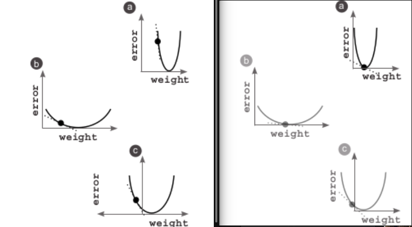
As in our previous example, we have three weights, so now let’s freeze a. So the basic observation would be the graph between error and weight is going to be shifted towards origin for a as the error is reducing because of other weights, but for a the weight is not modified. As we know the curve is the measure of each individual weight relative to the global error. So because of this at the end a is going to find the bottom of the bowl.
Gradient descent for multiple Output nodes
Ok so in the last topic we learned what to do if there are multiple inputs, now we’ll learn what to do if there are multiple outputs. So here we know we have a single input and multiple outputs and we also know $weight_delta = delta*input$.
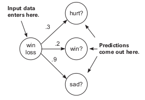
So here as we have multiple outputs which will result in individual deltas for each of the outputs multiplied with a single input to produce multiple weight deltas and hence different weight updates.
weights = [0.3, 0.2, 0.9]

def scalar_ele_mul(number,vector):
	output = [0,0,0]
	assert(len(output) == len(vector))
	for i in range(len(vector)):
		output[i] = number * vector[i]
	return output

def neural_network(input, weights):
	pred = ele_mul(input,weights)
	return pred

wlrec = [0.65, 1.0, 1.0, 0.9]

hurt = [0.1, 0.0, 0.0, 0.1]
win = [ 1, 1, 0, 1]
sad	= [0.1, 0.0, 0.1, 0.2]
input = wlrec[0]
true = [hurt[0], win[0], sad[0]]
pred = neural_network(input,weights)

error = [0, 0, 0]
delta = [0, 0, 0]
for i in range(len(true)):
	error[i] = (pred[i] - true[i]) ** 2
	delta[i] = pred[i] - true[i]

weight_deltas = scalar_ele_mul(input,weights)
alpha = 0.1
for i in range(len(weights)):
	weights[i] -= (weight_deltas[i] * alpha)
print("Weights:" + str(weights))
print("Weight Deltas:" + str(weight_deltas))
Gradient descent with multiple Input and Output nodes
Now as we learned about GD with multiple inputs and multiple outputs, we can easily frame it for multiple input and output NN.
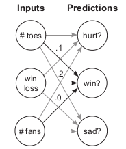
So here for handling this we need to take care of the matrices and other computations. So lets’ take one example -
- Input size = 3, matrix = [1,3]
- Output size = 3, matrix = [1,3] = true
- As all are interconnected so the size of the weight matrix will be [3, 3], and in python, it would of size 3 in the form of [ [1,3], [1,3], [1,3] ].
So as we know the first step will be making a prediction i.e. input*weight which will be getting a pred matrix of size 1,3.
After this, we will calculate delta i.e. pred - true. And after this, once we got delta we’ll calculate the weight delta with the help of normal matrix multiplication -
weight_delta = input*delta (here input size = [1,3] and delta is again [1,3]) so we’ll get the resultant matrix of [3,3] by the help of nested for loops. And once we got the matrix then we can easily calculate the weights update.
weights = [[0.1, 0.1, -0.3],
		   [0.1, 0.2,  0.0],
		   [0.0, 1.3, 0.1]]

def vect_mat_mul(vect,matrix):
	assert(len(vect) == len(matrix))
	output = [0,0,0]
	for i in range(len(vect)):
		output[i] = w_sum(vect,matrix[i])
	return output

def neural_network(input, weights):
	pred = ele_mul(input,weights)
	return pred

def outer_prod(vec_a, vec_b):
	out = zeros_matrix(len(a),len(b))
	for i in range(len(a)):
		for j in range(len(b)):
			out[i][j] = vec_a[i]*vec_b[j]
	return out

toes = [8.5, 9.5, 9.9, 9.0]
wlrec = [0.65,0.8, 0.8, 0.9]
nfans = [1.2, 1.3, 0.5, 1.0]

hurt = [0.1, 0.0, 0.0, 0.1]
win = [ 1, 1, 0, 1]
sad	= [0.1, 0.0, 0.1, 0.2]

alpha = 0.01
input = [toes[0],wlrec[0],nfans[0]]
true = [hurt[0], win[0], sad[0]]

pred = neural_network(input,weights)

error = [0, 0, 0]
delta = [0, 0, 0]
for i in range(len(true)):
	error[i] = (pred[i] - true[i]) ** 2
	delta[i] = pred[i] - true[i]

weight_deltas = outer_prod(input,weights)
for i in range(len(weights)):
	for j in range(len(weights[0])):
		weights[i][j] -= alpha * weight_deltas[i][j]
What actually these weights learn
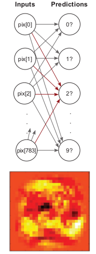
Let’s see this one more example based on the MNIST dataset, in this dataset, each data is 784 pixels i.e. (28 X 28). It’s called the Modified National Institute of Standards and Technology (MNIST) dataset, and it consists of digits that high school students and employees of the US Census Bureau handwrote some years ago. The interesting bit is that these handwritten digits are black-and-white images of people’s handwriting. Accompanying each digit image is the actual number they were writing (0–9). For the last few decades, people have been using this dataset to train neural networks to read human handwriting, and today, you’re going to do the same. And we have 10 labels that will help us to make predictions under a certain class. So as in the previous example, we saw a NN with multiple inputs and outputs so here we’ll apply this in this example i.e. input as 784 nodes and 10 outputs.
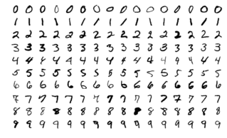
So instead of the input matrix as [1,3], we’ll have an input matrix of [1, 784]. and output as [1, 10]. As we know the image size is 28 X 28 so for converting it to [1, 784]. So for this, we’ll take the first row of pixels and concatenate them with the second row, and the third row, and so on, until you have one list of pixels per image.
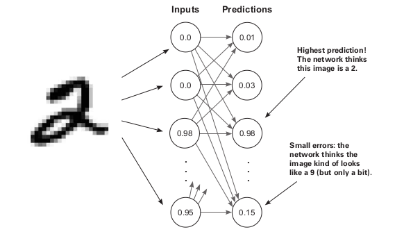
If the input is 2 then if predictions are exactly correct then the output would be 1 for 2 and 0 for others. So over this process, the network will adjust the weights and minimize the error.
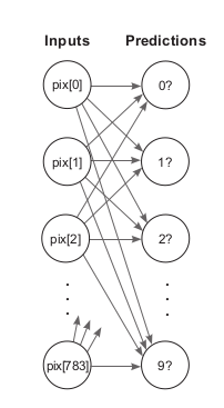
Well, if the weight is high, it means the model believes there’s a high degree of correlation between that pixel and the number 2. If the number is very low (negative), then the network believes there is a very low correlation (perhaps even negative correlation) between that pixel and the number 2. So if we plot, the pixels which have a high degree of correlation i.e. high weight it will should those pixels would be bright and others would be dark. So it happens because of good reason which we already learned i.e. because of DOT product. As we already know dot product tells us about the similarity which is there between two elements. if two vectors are almost similar then they have a high score of a dot product
So in next blog we’ll introduce Backward propagation….
Enjoy Reading This Article?
Here are some more articles you might like to read next: